Model
Our model employs the following principle: “The model dictates the inputs”. We recommend reading our introduction to have a better understanding of the PathLit model. A deeper look at the math used for the implementation is available in the optimisation page, under the Quant section.
caution
As the PathLit engine is currently in Alpha version, please do make sure you read the model assumption and the caveats section of this page.
Input Principle#
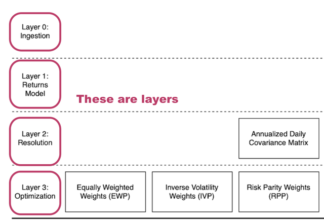
Blocks#
A block is a fundamental functional unit. An example of a block could be one that takes in a time series and outputs the daily log-returns. The blocks are organised into layers, and the blocks cannot exist on their own without an assignment to a layer. A block acts similarly to a function.
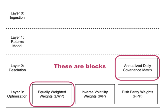
Layers#
A layer is a group of fundamental functional units (blocks) that takes the same input attributes and outputs the same attribute.
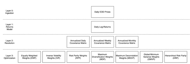
There are 3 layers in the current alpha version:
- Layer 1 (L1) is the Returns Model Generation layer. There is 1 block in this layer (l1r). This block generates daily returns from daily prices (Layer 0, i.e. L0) provided to the model.
| Layer | Block | Description |
|---|---|---|
| L1 | l1r | takes daily price data and computes the daily log-returns |
- Layer 2 (L2) is the Resolution Computation layer. There are 3 blocks in this layer (l2d, l2w,l2m). These blocks compute the annualised aggregated covariance matrix.
| Layer | Block | Description |
|---|---|---|
| L2 | l2d | takes the daily log-returns and computes the daily covariances between the assets |
| L2 | l2w | takes the daily log-returns and computes the weekly covariances between the assets |
| L2 | l2m | takes the daily log-returns and computes the monthly covariances between the assets |
- Layer 3 (L3) is the Optimisation layer. There are 7 blocks in this layer (l3ewp,l3ivp,l3rpp,l3mdp, l3mdcp, l3gmvp, l3hrp). These blocks define the asset weights to be computed for allocation.
| Layer | Block | Description |
|---|---|---|
| L3 | l3ewp | takes the covariances between the assets and computes the equally-weighted portfolio weights |
| L3 | l3ivp | takes the covariances between the assets and computes the inverse-volatility weighted portfolio weights |
| L3 | l3rpp | takes the covariances between the assets and computes the risk-parity weighted portfolio weights |
| L3 | l3mdp | takes the covariances between the assets and computes the maximum diversification weighted portfolio weights |
| L3 | l3mdcp | takes the covariances between the assets and computes the maximum decorrelation weighted portfolio weights |
| L3 | l3gmvp | takes the covariances between the assets and computes the global minimum-variance weighted portfolio weights |
| L3 | l3hrp | takes the covariances between the assets and computes the hierarchical risk-parity weighted portfolio weights |
There are 1 + 3 + 7 = 11 computational blocks. Given the 11 blocks, there are 1 x 3 x 7 = 21 computational paths, since there are no repeated or disallowed paths for now.
Paths#
A path is the interconnection between the blocks in every layer. They are indicated in the outputs in the following structure:
l1[a].l2[b].l3[c]
As more blocks and layers are added, the definition of the path will expand to reflect that change, but in a structure not too dissimilar from the examples given below:
l1[a].l2[b].l3[c].l4[d].l5[e]…Examples#
l1r.l2d.l3ewp entails that the daily price data that has been provided has first been:
- [
l1r] converted into daily log-returns, then; - [
l2d] converted into the daily covariances between the assets, then; - [
l3ewp] allocated weights that are computed based on the equally-weighted portfolio strategy.
l1r.l2m.l3hrp entails that the daily price data that has been provided has first been:
- [
l1r] converted into daily log-returns, then; - [
l2m] converted into the monthly covariances between the assets, then; - [
l3hrp] allocated weights that are computed based on the hierarchical risk-parity weighted portfolio strategy.
We use this model to dictate the roadmap for developing the blocks and layers. This helps us to remain parsimonious with the inputs. We currently only use the covariance structure of the log-returns of the assets provided. Thus, the current model is simple and subjected to small estimation errors, but large biases. We will expand the inputs to include:
- Future release
- expected returns
- user constraints on individual assets
- box constraints on asset classes
Given that all L3 optimisation blocks require the covariance matrix, the annualised log-returns of the instruments are required to compute them. There are 3 methods in which annualised log-returns could be computed: they can be aggregated from either a i) daily, ii) weekly or iii) monthly resolution. Thus L2 contains 3 blocks addressing each resolution above, and the aggregated log-returns only requires daily returns and that one and only block is in L1.
This methodology keeps inputs precise, while offering multiple paths.
Path Independence#
With currently 3 layers and 11 blocks, there are a total of 21 paths that the algorithm is able to traverse.
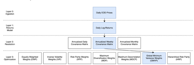
A particular example is as follows:
Ingest a Time Series of 3 assets-> Convert to daily log-returns-> Annualise from weekly log-returns-> Churn out weights according to the Global Mean Variance (GMVP) Framework.This is 1 of 21 paths.
Because we do not dictate which path is the best, we present the weights generated by all 21 paths to the user for decision and sense-making. This creates an un-opinionated optimisation tool, as we describe it in the introduction page
However, we understand that for better sense-making, a preliminary ranking structure is required besides the weights. For this, a backtesting module with simulated data generated using Monte Carlo is used to provide portfolio performances in dollar terms for all the paths. This can be accessed using the /sims endpoint.
Model Assumptions#
The model is kept simple with the assumptions that:
The model is independent and identically distributed (i.i.d.) for any length of time series that is provided as the input.
It does not take discontinuous datasets, thus it is able to process ETFs, Mutual Fund and Stocks only for now. More instruments are to come with further releases of the PathLit engine.
The model does not make any assumptions about stationarity nor if any volatility clustering is exhibited by the time series that is provided as the input.
The model only takes the covariance matrix as an input for the initial alpha release of the PathLit engine, thus the choice of optimisers in L3 are limited to Heuristic (EWP, IVP), Risk-Based (RPP, MDP, MDCP, HRP) and Mean-Variance (GMVP) optimisation frameworks.
Caveats#
The PathLit engine is in early alpha, some caveats for the model algorithm include:
- For inputs that can take constraints on the instruments, a lower bound of 0 and an upper bound of 1 is taken, i.e. only portfolio with no short-selling and long-only constraints are generated only
- As some optimisers are notorious for generating corner solutions, for example, GMVP, which would generate portfolios which allocates weights to only a few assets, care must be taken when deciding if this strategy is suitable for your needs.