R
Using the Package#
Pre-requisite: A PathLit account is required to interact with the API with a unique key to the account. It can be created at the account creation page.
PathLit R package on CRAN#
Traditionally, R Packages live in the Comprenhensive R Archive Network - CRAN in short. We are working towards having a version of this SDK there to make it as easy as possible to use in an R project.
Installation (from CRAN)#
library(devtools) install.packages("pathlit")
* installing *source* package ‘pathlit’ ...** package ‘pathlit’ successfully unpacked and MD5 sums checked** using staged installation** R** byte-compile and prepare package for lazy loading** help*** installing help indices** building package indices** testing if installed package can be loaded from temporary location** testing if installed package can be loaded from final location** testing if installed package keeps a record of temporary installation path* DONE (pathlit)Documentation#
There are function level documentation available using the standard R help operator: help() or ?
?[function_name] ?get_info help(get_info)Tutorial#
Objective#
In this quick tutorial, we are going to install the PathLit R package (command line or the R Studio IDE), query the paths endpoint with three tickers "AAPL", "MSFT", "HD". paths computes the dollar returns of a portfolio for the actual time series (e.g. using the realised market data), plot two strategies (l1r.l2d.l3hrp and l1r.l2d.l3mdcp (what is this?).
Finally we'll use the sims endpoint which computes the dollar returns of a portfolio for multiple simulated time series (e.g. the simulated market data) apply three runs for our three tickers ("AAPL", "MSFT", "HD"), two strategies (l1r.l2d.l3hrp and l1r.l2d.l3mdcp) and plot them.
Let's do it#
Step 1: Set-up an account with us and retrieve and API Key. For the purposes of this tutorial, we will use a dummy key: 56gIvzm4dj1vJpNUlv3RJ2CeMd47JETG3bcf5zLS.
Step 2: Install the required packages to run this tutorial (if you don't already have them). We need the CRAN package xts to be able to work with time series later when plotting our charts.
install.packages('xts')
Step 3: Initialise the package and register the key:
library(pathlit) Client("56gIvzm4dj1vJpNUlv3RJ2CeMd47JETG3bcf5zLS")Step 4: Retrieve the list of available tickers, in order to select a few for analysis:
get_tickers()Step 5: View the time series of the tickers selected e.g.
AAPL, MSFT and HD:
    tickers <- c("AAPL", "MSFT", "HD")    ts <- get_timeseries(tickers)    na.omit(ts)
    plot(ts,         main = "Time Series Data",         xlab = paste0(as.character(start(ts)), " - ", as.character(end(ts)))    )
Step 6: Obtain the weights of the tickers selected, via our existing strategies. Please note that even though for this tutorial we chose to focus on two strategies (l1r.l2d.l3hrp and l1r.l2d.l3mdcp), the get_weights(tickers) function will return all the current PathLit suported strategies.
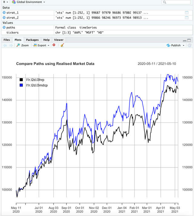
get_weights(tickers)Step 7: Obtain the paths of our existing strategies of the tickers selected, using the realised market data, for a staring portfolio of USD 100,000:
    paths <- get_paths(tickers)
    strat_1 <- xts::as.xts(paths[, 3]) # l1r.l2d.l3hrp    strat_2 <- xts::as.xts(paths[, 5]) # l1r.l2d.l3mdcp
library(xts) plot.xts( cbind(strat_1, strat_2), col = c("black", "blue"), legend.loc = "topleft", main = "Compare Paths using Realised Market Data" )You should get something like this:
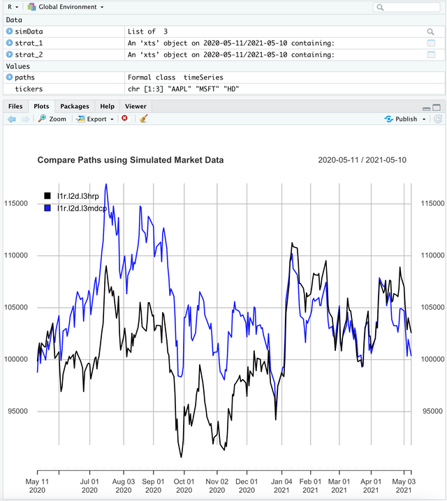
Step 8: Obtain the paths of our existing strategies of the tickers selected, using 3 simulated market data runs, for a staring portfolio of USD 100,000:
    simData <- Simulate(tickers, 3)    strat_1 <- xts::as.xts(simData[[2]][, 3]) # l1r.l2d.l3hrp from the 2nd run    strat_2 <- xts::as.xts(simData[[2]][, 5]) # l1r.l2d.l3mdcp from the 2nd run
plot.xts( cbind(strat_1, strat_2), col = c("black", "blue"), legend.loc = "topleft", main = "Compare Paths using Simulated Market Data" )Which should give you something similar to that:
Conclusion#
At the end of this quick tutorial, you:
- Installed the PathLit
Rpackage from the CRAN repository - (optionally) retrieved the currently supported tickers by the PathLit Engine
- Computed the weights for thre tickers (
"AAPL", "MSFT", "HD") and two strategies (l1r.l2d.l3hrpandl1r.l2d.l3mdcp) - Computed and plotted the dollars returns of a USD 100,000 with realised market data for these three tickers and two strategies (a form of backtesting)
- Computed and plotted the dollars returns of a USD 100,000 with three simulated market data runs for these three tickers and two strategies (a form of risk simulation AKA Monte Carlo simulation).
What's next?#
You could modify your code to plot all the strategies currently supported by the PathLit Engine for these three tickers and observe which one is better than the others given the context of these three tickers.
If you have a personal/proprietary strategy, you could benchmark it against the currently supported strategies by the PathLit Engine and get some meaningful perspectives.
If you are code savvy you could even build an active robo-advisor using the the PathLit Engine to compute the allocation of the stocks you wish to see in one or many portfolio.